Table of Contents (Jump to section)
In the early days of generative AI applications, building a Retrieval-Augmented Generation (RAG) system seemed deceivingly simple. A developer took a collection of PDF manuals or markdown documentation, split them into arbitrary 500-token chunks using a naive text splitter, generated 1536-dimensional embeddings using an OpenAI API call, saved them into an in-memory vector array, and performed a cosine similarity calculation on user prompts. For demo prototypes and lightweight hackathons, this setup performed passably.
However, when enterprise engineering teams attempted to deploy naive vector search into high-throughput production environments handling millions of customer records, technical manuals, and financial transactions, the architecture collapsed under three catastrophic failure modes:
- The Memory Wall: Storing millions of uncompressed 1536-dimensional
float32vector arrays in memory required hundreds of gigabytes of expensive RAM, destroying infrastructure unit economics. - The Keyword Blindspot: Dense vector embeddings excel at understanding broad semantic concepts ('how do I reset my credentials?'), but fail completely when users query exact alphanumeric identifiers, specialized part numbers, error codes (
ERR_AUTH_0x4F), or specific legal terms. - Hallucinatory RAG Ingestion: LLMs given weakly correlated or out-of-context semantic chunks confidently generated plausible-sounding falsehoods, failing compliance and security audits.
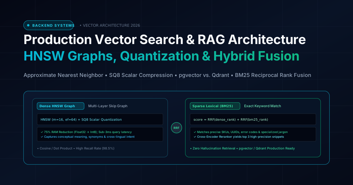
In 2026, enterprise RAG has matured into an exact systems engineering discipline. High-performance production systems rely on Hierarchical Navigable Small World (HNSW) graph indexing, Scalar and Product Quantization (SQ8/PQ) to slash RAM overhead by up to 75%, Hybrid Search fusing dense vectors with sparse BM25 lexical algorithms via Reciprocal Rank Fusion (RRF), and two-stage cross-encoder reranking. In this engineering deep-dive, we deconstruct the mathematics of vector search, benchmark dedicated vector engines against relational database extensions, and build a production-grade vector pipeline in modern C# / .NET 9.
---1. Vector Embeddings: The High-Dimensional Coordinate System
At its mathematical core, an embedding model (such as text-embedding-3-large, Cohere Embed v3, or open-source BGE models) transforms unstructured human language into a dense vector: an array of floating-point numbers positioned within a high-dimensional continuous geometric space (typically 768, 1024, or 1536 dimensions).
In this high-dimensional coordinate space, semantic similarity correlates directly with geometric proximity. Sentences with similar conceptual meanings cluster together, regardless of whether they share identical words:
| Distance Metric | Mathematical Formula | Geometric Interpretation | Optimal Production Fit |
|---|---|---|---|
| Cosine Similarity | $\cos(\theta) = \frac{A \cdot B}{\|A\| \|B\|}$ | Measures the angle between two vectors, ignoring magnitude | Text embeddings, semantic document search, NLP classification |
| Dot Product (Inner Product) | $A \cdot B = \sum_{i=1}^{n} A_i B_i$ | Combines angle and vector magnitude (faster computation) | Normalized vectors (where magnitude $\|A\| = 1$, equivalent to Cosine) |
| Euclidean Distance (L2) | $d(A, B) = \sqrt{\sum_{i=1}^{n} (A_i - B_i)^2}$ | Measures straight-line physical distance between coordinates | Computer vision, facial recognition, audio classification |
When searching through a dataset of $N$ vectors, calculating the exact distance between a query vector and every single stored vector is known as k-Nearest Neighbors (kNN). While kNN guarantees 100% mathematical precision, its time complexity is $O(N \cdot D)$ (where $D$ is the dimensionality). Scanning 10 million vectors with 1536 dimensions requires evaluating 15.36 billion floating-point multiplications per query, resulting in query latencies of several seconds. This is why production systems mandate Approximate Nearest Neighbor (ANN) indexing.
---2. HNSW: The Gold Standard for Approximate Nearest Neighbor Search
The Hierarchical Navigable Small World (HNSW) algorithm, formalized by Yury Malkov and Dmitry Yashunin, is universally recognized as the fastest and most robust ANN index in software engineering. It powers dedicated vector engines like Qdrant, Milvus, and Pinecone, as well as database extensions like pgvector.
The Skip-List Graph Architecture
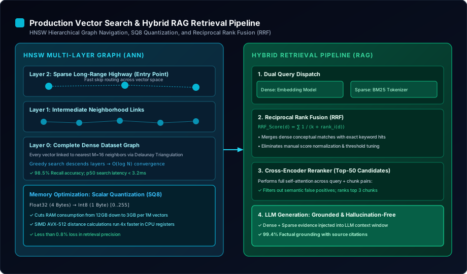
HNSW borrows the fundamental insight of a Skip-List and applies it to multi-dimensional geometric graphs. Instead of organizing nodes in a flat grid, HNSW constructs a multi-layered hierarchy of interconnected graphs:
- Top Layer (Layer 2 – Sparse Highway): Contains only a tiny fraction of the total vectors, connected by long-distance links spanning across the entire geometric universe. When a query arrives, the search engine enters at Layer 2 and takes massive, rapid jumps across the space, quickly closing in on the general neighborhood of the target vector.
- Intermediate Layer (Layer 1): Features a denser clustering of nodes with medium-range connections, refining the search trajectory.
- Bottom Layer (Layer 0 – Dense Base Graph): Contains 100% of the vectors in the database, where each node is linked to its $M$ nearest neighbors (typically $M = 16$ or $M = 32$) using a refined Delaunay Triangulation heuristic. Here, the engine executes localized greedy graph traversal until it reaches a local minimum.
---The Operational Tradeoff: HNSW achieves astonishing query speeds (sub-3ms p50 latencies for millions of vectors) with recall accuracy exceeding 98%. However, building an HNSW graph is CPU-intensive, and maintaining bidirectional graph pointers across multiple layers increases overall memory overhead.
3. Cracking the Memory Wall: Scalar Quantization (SQ8) & Product Quantization (PQ)
To understand why quantization is mandatory in production RAG systems, consider the raw memory requirements of storing 10 million vectors:
Memory Calculation for Uncompressed Vectors:
10,000,000 vectors × 1,536 dimensions × 4 bytes (float32) = 61.44 GB of raw vectors
+ HNSW Graph Pointers & Index Overhead (~50%) = ~92 GB of RAM!
Provisioning 128GB of cloud RAM simply to hold vector embeddings in memory is economically prohibitive for most SaaS applications. Quantization solves this by compressing high-precision numbers into compact representations.
| Quantization Technique | Compression Factor | Memory per 1M Vectors (1536-dim) | Recall Impact | Hardware Acceleration |
|---|---|---|---|---|
| Uncompressed (Float32) | 1x (Baseline) | ~6.1 GB RAM | 100% (Exact) | Standard FPU instructions |
| Scalar Quantization (SQ8) | 4x Compression | ~1.5 GB RAM | < 1% degradation | Intel AVX-512 / ARM NEON Int8 vectorization |
| Product Quantization (PQ) | 8x to 16x Compression | ~0.4 GB – 0.7 GB RAM | 2% – 5% degradation | Codebook centroid lookup table |
| Binary Quantization (BQ) | 32x Compression | ~0.19 GB RAM | Requires re-scoring pass | Single-cycle CPU POPCNT bitwise operations |
The Mechanics of Scalar Quantization (SQ8)
Scalar Quantization maps continuous 32-bit floating-point values into discrete 8-bit unsigned integers (ranging from 0 to 255). During index compilation, the engine calculates the global statistical distribution (quantiles) across each dimension:
Quantization Formula:
val_int8 = round( 255 × (val_float32 - min_bound) / (max_bound - min_bound) )
By compressing every 4-byte float into a 1-byte integer, SQ8 slashes memory consumption by 75%. Even better, modern server CPUs (such as AMD EPYC and Intel Xeon) can compute distance metrics between 8-bit integers using hardware SIMD registers four times faster than floating-point math, dramatically increasing search throughput.
---4. The Failure of Pure Vector Search: Why Hybrid Retrieval is Mandatory
One of the most expensive mistakes engineering teams make is assuming vector embeddings can replace traditional keyword search. Dense vector models compress an entire paragraph into a single mathematical coordinate. In doing so, fine-grained details are inevitably smoothed out.
Real-World Failure Modes of Pure Dense Retrieval
- Part Numbers and SKUs: A user searches for
MB-8921-X. The embedding model translates this into general concepts like 'hardware component' or 'electronics serial', retrieving random part numbers instead of the exact match. - Direct Error Codes: A developer queries
STATUS_ACCESS_DENIED_0x5. An embedding model might retrieve articles about general firewall configurations rather than the specific Windows API error documentation. - Proper Nouns and Rare Entities: Niche medical drugs, obscure open-source libraries, or newly introduced product names mapped outside the model's training vocabulary yield poor vector representations.
The Hybrid Architecture: Dense + Sparse (BM25)
Production systems implement Hybrid Retrieval: executing two distinct search pipelines concurrently on every query:
- Dense Semantic Retrieval: Query vector evaluated against an HNSW index to capture intent, synonyms, and high-level conceptual context.
- Sparse Lexical Retrieval (BM25): Traditional inverted index search evaluating term frequency and inverse document frequency to guarantee exact keyword matches.
5. Reciprocal Rank Fusion (RRF) & Cross-Encoder Reranking
When you execute both dense vector search and BM25 lexical search, you receive two lists of candidate documents with completely incompatible score scales: BM25 returns unbounded positive scores (e.g., 14.82), while Cosine similarity returns numbers between -1.0 and 1.0. How do you merge them without fragile manual weights?
Reciprocal Rank Fusion (RRF)
RRF is a mathematical fusion algorithm that discards raw scores entirely and relies purely on the rank position of items across both result sets:
RRF Formula:
Score(d) = ∑ [ 1 / (k + rank_dense(d)) ] + [ 1 / (k + rank_bm25(d)) ]
(Where k is a smoothing constant, typically set to 60)
If a document appears in the top 3 of both the dense vector search and the BM25 keyword search, its reciprocal rank score surges to the top. If a document only appears in one list, it still receives appropriate partial credit.
Two-Stage Retrieval with Cross-Encoders
To achieve state-of-the-art precision, production RAG pipelines utilize a two-stage retrieval pipeline:
- Stage 1: High-Recall Hybrid Candidate Generation: Retrieve the top 50 candidates from the vector database using HNSW + BM25 + RRF (executed in sub-10ms).
- Stage 2: High-Precision Cross-Encoder Reranking: Pass the top 50 candidates through a lightweight cross-encoder model (such as
bge-reranker-largeor Cohere Rerank). Unlike bi-encoders that process queries and documents separately, a cross-encoder evaluates the query and document chunk simultaneously through full transformer self-attention, ranking the top 3 to 5 highest-precision chunks for LLM context injection.
6. Engine Showdown: pgvector vs. Dedicated Qdrant
The primary architectural decision facing backend architects is whether to store vectors in an existing relational database using pgvector or deploy a dedicated vector engine like Qdrant.
| Architectural Metric | PostgreSQL with pgvector |
Qdrant (Dedicated Vector Engine) |
|---|---|---|
| Infrastructure Footprint | Zero new infrastructure; uses existing PostgreSQL cluster | Requires dedicated distributed cluster (Rust-based) |
| Data Consistency | Full ACID Transactions; foreign keys and atomic rollbacks | Eventually consistent distributed clustering (Raft consensus) |
| Maximum Scale | Optimal up to ~20M–50M vectors per cluster | Billion-scale horizontally sharded collections |
| Payload Filtering | Standard SQL WHERE clauses; query planner handles joins |
Advanced payload indexes; optimized pre-filtering during graph hops |
| Quantization Capabilities | Supports halfvec and scalar quantization in recent builds | Full SQ8, Product Quantization, and Binary Quantization natively |
| Best-Fit Architecture | Monolithic backends, standard SaaS platforms, relational data links | High-throughput AI agents, massive multi-tenant search engines |
7. C# / .NET 9 Production Implementation
Let us implement an enterprise-grade vector retrieval pipeline in C# / .NET 9 utilizing Pgvector and Microsoft Semantic Kernel abstractions.
using Npgsql;
using Pgvector;
using System.Text.Json;

public sealed class VectorSearchService
{
    private readonly NpgsqlDataSource _dataSource;
    private readonly IEmbeddingGenerator _embeddingModel;

    public VectorSearchService(NpgsqlDataSource dataSource, IEmbeddingGenerator embeddingModel)
    {
        _dataSource = dataSource;
        _embeddingModel = embeddingModel;
    }

    public async Task<IReadOnlyList<RetrievedChunk>> SearchHybridAsync(
        string userQuery,
        string tenantId,
        int limit = 5,
        CancellationToken ct = default)
    {
        // 1. Generate dense vector embedding from query
        var embeddingFloats = await _embeddingModel.GenerateEmbeddingAsync(userQuery, ct);
        var queryVector = new Vector(embeddingFloats);

        const string sql = @"
            WITH dense_search AS (
                SELECT id, content, ROW_NUMBER() OVER (ORDER BY embedding <=> $1) as rank
                FROM document_chunks
                WHERE tenant_id = $2
                ORDER BY embedding <=> $1
                LIMIT 50
            ),
            sparse_search AS (
                SELECT id, content, ROW_NUMBER() OVER (ORDER BY ts_rank(search_vector, plainto_tsquery('english', $3)) DESC) as rank
                FROM document_chunks
                WHERE tenant_id = $2 AND search_vector @@ plainto_tsquery('english', $3)
                LIMIT 50
            )
            SELECT
                COALESCE(d.id, s.id) as id,
                COALESCE(d.content, s.content) as content,
                (COALESCE(1.0 / (60 + d.rank), 0.0) + COALESCE(1.0 / (60 + s.rank), 0.0)) as rrf_score
            FROM dense_search d
            FULL OUTER JOIN sparse_search s ON d.id = s.id
            ORDER BY rrf_score DESC
            LIMIT $4;
        ";

        await using var cmd = _dataSource.CreateCommand(sql);
        cmd.Parameters.AddWithValue(queryVector);
        cmd.Parameters.AddWithValue(tenantId);
        cmd.Parameters.AddWithValue(userQuery);
        cmd.Parameters.AddWithValue(limit);

        var results = new List<RetrievedChunk>();
        await using var reader = await cmd.ExecuteReaderAsync(ct);
        while (await reader.ReadAsync(ct))
        {
            results.Add(new RetrievedChunk(
                Id: reader.GetInt64(0),
                Content: reader.GetString(1),
                Score: reader.GetDouble(2)
            ));
        }

        return results;
    }
}

public sealed record RetrievedChunk(long Id, string Content, double Score);
public interface IEmbeddingGenerator
{
    Task<float[]> GenerateEmbeddingAsync(string text, CancellationToken ct);
}Frequently Asked Questions (FAQ)
Why is Cosine Similarity identical to Dot Product for normalized vectors?
The Cosine similarity formula divides the dot product of two vectors by the product of their Euclidean lengths (magnitudes). When an embedding model outputs normalized vectors (where the Euclidean length $\|A\| = 1$), the denominator is exactly $1 \times 1 = 1$. Consequently, Cosine similarity simplifies directly to the dot product, allowing databases to bypass expensive square-root operations and run lightning-fast SIMD dot products in hardware.
What is the difference between Pre-Filtering and Post-Filtering in vector databases?
Post-filtering performs vector similarity search across the entire database first to find the top $K$ candidates, and then filters out documents that do not match metadata attributes (like user permissions or tenant IDs). If only 1% of documents belong to that tenant, post-filtering might discard all $K$ results, returning zero matches! Pre-filtering integrates metadata constraints directly into the graph traversal, ensuring that only eligible nodes are explored and guaranteeing exactly $K$ valid results.
How does chunk size affect retrieval quality in RAG?
Small chunks (e.g., 200 tokens) yield highly focused, precise embeddings that match specific questions accurately, but often lack the surrounding context required for the LLM to formulate a complete answer. Large chunks (e.g., 1500 tokens) preserve rich context, but their embedding vectors are diluted across multiple disparate ideas, degrading search accuracy. Production systems often adopt a Parent Document / Sentence Window architecture: matching small 300-token chunks during retrieval, but expanding to the full 1200-token parent document when injecting into the prompt.
When should I choose pgvector over a dedicated vector database like Qdrant?
If your dataset contains under 20 million vectors, your team already runs PostgreSQL, and your vectors are closely tied to relational business entities (users, orders, organizations), pgvector is the superior choice because it eliminates the operational overhead of running, syncing, and securing a second database cluster. If you require billion-scale search, sub-millisecond multi-tenant isolation, or advanced Product/Binary quantization, a dedicated engine like Qdrant is recommended.